Navigation is important for the plot area (that's the area where the data graph is displayed). There are several possible ways of navigation:
- Keyboard navigation
Use the Left and Right cursor keys for slow navigation and the Page Up and Page Down key for fast navigation. Use Home and End to get to the start or to the end of the display area.
To support markers, the Ctrl+Left or Ctrl+Right shortcut can be used to jump to the left or right marker.
- Toolbar
The toolbar also has items for navigation: Use the Left and Right icon to navigate slow, the Page left and Page right icon to navigate fast and the Begin and End icon to navigate to the top or bottom of the data area.
- Scrollbar
You should be familar how to use a scrollbar. However, note that while dragging the slider the display is not updated. This is because of performance reasons if the displayed area is large.
- Mouse wheel
If you have a wheel mouse, it's very easy to navigate. Just rotate the mouse wheel to move forward/backward in the timeline or press the Shift key while roatating to move faster.
- Menu entries
The menu holds the whole functions as menu items. This items are not intended to used by choose them from the menu but they are provided to present the keyboard shortcuts in a common way to the user.
Only the and items may be accessed directly.
- Keyboard zooming
Use + to zoom in, - to zoom out, F2 to come back to the default zoom factor, F3 to fit the whole data on the display and F4 to fit the marked data (markers are discussed later) on the screen.
- Toolbar
Use Zoom In to zoom in, Zoom Out to zoom out, Zoom Default to come back to the default zoom factor, Zoom Fit to fit the whole data on the display and Zoom to fit markers to fit the marked data (markers are discussed later) on the screen.
- Mouse wheel
If you hold the Ctrl key while rotating the mouse wheel, scrolling is performed. For other scrolling actions use the toolbar, the keyboard or the menu entries.
- Menu entries
The menu holds the whole functions as menu items. This items are not intended to used by choose them from the menu but they are provided to present the keyboard shortcuts in a common way to the user.
Markers (TFLA-01 provides two of them) are useful in much situations:
To show the (mostly) exact time of a certain point in the plot area. The time cannot be exact because we don't use realtime capabilities of the operating system (neither "normal" Linux now Windows have hard realtime capabilities) but it is accurate enough in most situations.
To show a time difference between two measuring points.
To remember a position in the data area while scrolling to another position for a short while.
To help for zooming: Just select the area you want to see more detailled and press F4 or use the Zoom to fit markers.
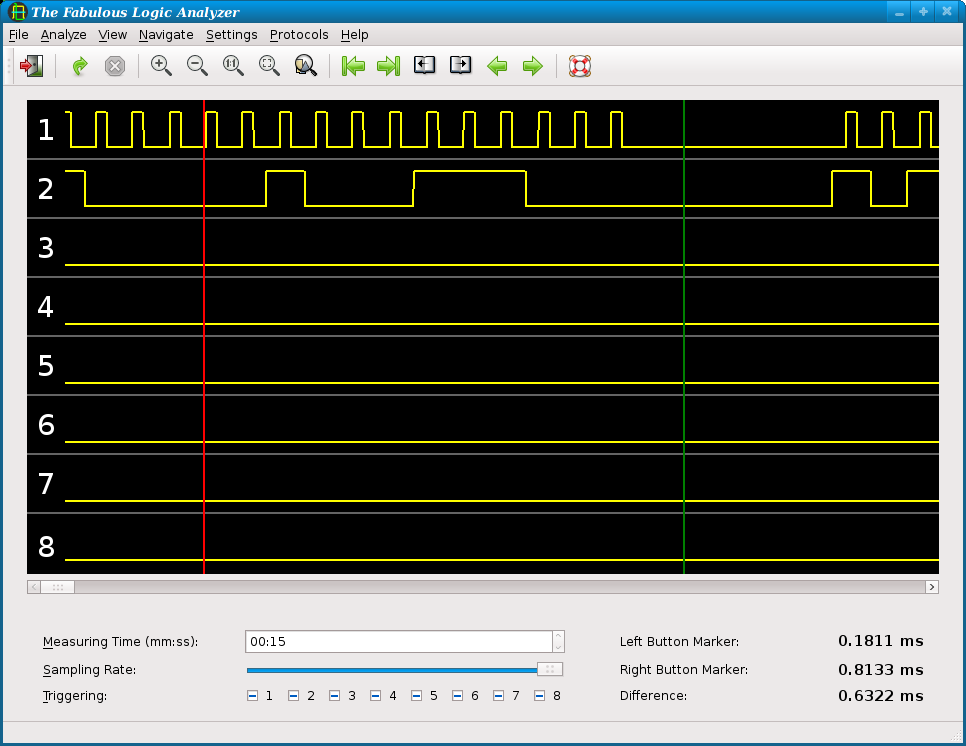
TFLA-01 supports a so-called left marker and a right marker. To set markers, click on the plot area with the left or the right mouse button. The left marker is intended to be left of the right marker, but it must not. If not, the time difference is negative. See Navigation to see how markers can be used to navigate and Zooming for information about scrolling and markers.
Triggering is useful if you want to monitor a line for a longer period of time and you mostly wait for an event to occure. For example you are alone and you have to start the logic analyzer to monitor data and you also have to do some manual steps to start the action on the data lines to occure.
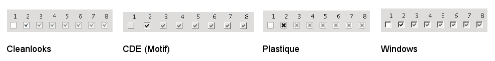
For each line you can configure if the line should be low or high to trigger of if the line should be ignored. If all lines are set to ignore, triggering is disabled. The display of the three states may depend of the GUI style of Qt, the screenshot shows the Cleanlooks, Motif/CDE, Plastique and Windows style. The first line is set to trigger on low level, the second on high level and all other lines are ignored.
Note
Triggering may not work if the period where the value which should be triggered for is two low. Since the function which waits for the triggered data is a part of the libieee1284 parallel port library, we have no influence on this.
Also, triggering may be implemented differently on the operating system. For example on Linux it's part of the kernel module which means that there's no CPU usage until the triggered value is detected.
The measuring time sets the time to sample data after the user clicked on Start and if he doesn't Stop. Note that depending on the system speed the quantity of data is large so the same is for the memory consumtion (expect 1 MByte per second). Also the GUI is slow if drawing large data areas in this situation. So normally, a timespan between 1 and 10 seconds is a good idea.
It's possible to save the data that has been collected with TFLA-01 in an application-specific, binary format that can be opened with TFLA-01 again. The format is platform an machine independent, so a file that has been saved on a SPARC Solaris machine can be read on a Intel Windows machine and vice versa.
To save the data, use → . The default extension is dat. To read the file again, choose → . To open the last file after the application has been restarted, you can also use → .
The current plot can be saved as image with → . Currently, exaclty the displayed area is saved including the markers and the only supported format is PNG. This may change in future.
The current data can be exported as CSV (comma separated value) with → . Each sample is a line and each bit is a column. This can be used with in a spreadsheet application like OpenOffice.org or in custom scripts.
After the file has been selected, you will be asked if only the state changes should be saved. If you choose , then only the data sets will be saved where something changed. This reduces the file size dramatically.
Starting with version 0.3.0, a tiny I²C analyzer has been integrated. This is a contribution by Jose Aparicio
(<aparicio@lip.pt>). And with 0.4.0, even an analyzer for SPI has been integrated which has been
contribued by Kai Dorau (<kai.dorau@gmx.net>). Both analyzers share a common user interface which
is explained below.
At first you have to tell the software which of your input channel represents which logic channel of the bus protocol. While I²C has the two lines SDA and SCL (data and clock), SPI has SDI (MOSI), SDO (MOSI) and SCK (data in, data out and clock). The SPI decoder supports only one data direction at a given time.
To do the assignment, choose → . Then a dialog as shown below should appear.
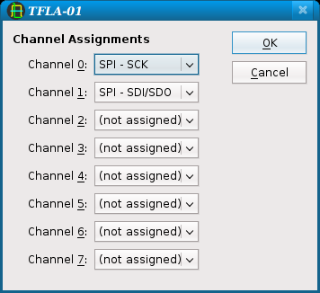
In this dialog, it's possible to assign a protocol channel for each input channel.
If all protocol channels of a given protocol have been assigned, the corresponding entry in the menu should be enabled. To do the actual decoding, just select → or → . After a short while, the result should be displayed in a dialog as shown below:
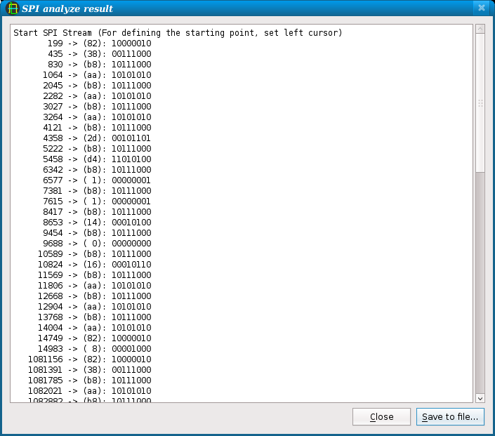
Just choose to save the contents of that result dialog to a file.
Note
If you don't want to analyze the whole data set, just use the markers to select a start and end position. In that case, only the selected data set will be analyzed.